Weighting For All Calculations
The Weighting Values (Weight #1 (%)…) is used to assign weights to each input, thus allowing each momentum or volatility or Sharpe ratio or Information Ratio to be assigned different weight values. For example say you would like to make a position score depend 25% on 3 month momentum and 25% on 4 month volatility and 50% on 6 month Sharpe Ratio. You would select the appropriate weight values under each section corresponding to the momentum/volatility/sharpe ratio length to allow for this allocation. When calculating the position score or other metric the weight value then determines the final position score based on 25% momentum, 25% volatility, and 50% Sharpe Ratio as you setup the simulation to run.
Momentum Calculations
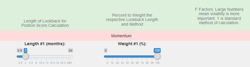
Momentum is defined for our tools as the return % over a specific time frame [Momentum = 100 * (Price Today – Price X Months Ago) / Price Today].
Therefore the length of the momentum is how far we lookback in time (in months, where 1 month = 22 days). So the 3 month momentum of a security in % = the price today minus the price 3 months ago divided by the price today. If ‘Actual Months’ is selected an actual month (1-1 to 2-1) is used instead of the average 22 days per month.
Example: SPY currently has a price of 200 and had a price 3 months ago of 190, TLT has a price of 130 currently and had a price of 120 3 months ago.
SPY 3 Month Momentum = 100 * (Price Today – Price 3 Months Ago) / Price Today = 100 * (200 – 190) / 200 = 5%
TLT 3 Month Momentum = 100 * (Price Today – Price 3 Months Ago) / Price Today = 100 * (130 – 120) / 130 = 7.6923%
Therefore TLT had the higher 3 month momentum, therefore for a rotation strategy TLT would be chosen over SPY for this period.
Volatility Calculations
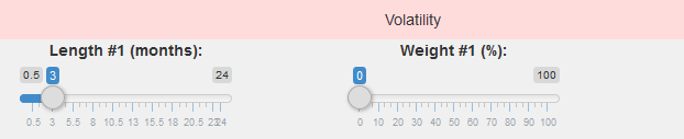
Volatility is defined for our tools as the standard deviation of a securities returns over a specific time frame [Volatility = Standard Deviation of Rate of change of the securities returns].
Therefore the length of the volatility is how far we lookback in time (in months, where 1 month = 22 days). So the 3 month volatility of a security in % = the standard deviation of that securities returns over a 3 month period.
Sharpe Ratio Calculations
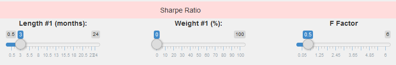
The Sharpe Ratio is defined for our tools as the average of the daily returns over a specific time frame divided by standard deviation of a securities returns over a specific time frame [Sharpe Ratio = average of Securities X Month Daily Returns / (Standard Deviation of Rate of change of the securities returns over X Months) ^ Volatility Factor].
The Volatility Factor (sometimes called F Factor) is not a part of the original Sharpe Ratio calculation, if this value is set to 1 the calculation will use the default Sharpe Ratio calculation methods. The Volatility Factor can be changed to adjust how important the volatility (standard deviation of the securities returns) is in the calculation of the Sharpe Ratio. If it is set to a low value the volatility value is small therefore the Sharpe Ratio will be closer to a momentum only strategy; if the volatility factor is set high then the strategy takes into account the volatility of the security much more so it is closer to a volatility only strategy.
Therefore the length of the Sharpe Ratio is how far we lookback in time (in months, where 1 month = 22 days). So the 3 month Sharpe Ratio of a security = Average Daily Return over 3 Months / (Volatility over 3 Months ^ F_Factor).
Information Ratio Calculations
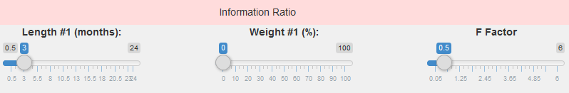
The Information Ratio is defined for our tools as the returns over a specific time frame divided by standard deviation of a securities returns over a specific time frame [Information Ratio = Securities X Month Return / (Standard Deviation of Rate of change of the securities returns over X Months) ^ Volatility Factor]. So the Information Ratio is essentially the Momentum / Volatility where volatility is raised to a power (volatility factor or f factor).
The Volatility Factor (sometimes called F Factor) is not a part of the original Information Ratio calculation, if this value is set to 1 the calculation will use the default Information Ratio calculation methods. The Volatility Factor can be changed to adjust how important the volatility (standard deviation of the securities returns) is in the calculation of the Information Ratio. If it is set to a low value the volatility value is small therefore the Information Ratio will be closer to a momentum only strategy; if the volatility factor is set high then the strategy takes into account the volatility of the security much more so it is closer to a volatility only strategy.
Therefore the length of the Information Ratio is how far we lookback in time (in months, where 1 month = 22 days). So the 3 month Information Ratio of a security = Momentum over 3 months / Volatility over 3 months ^ F_Factor.
Variance Calculations
Variance is defined for our tools as the average of the daily return squared divided by the number of terms in the calculation.
Therefore the length of the variance is how far we lookback in time (in months, where 1 month = 22 days). So the 3 month variance of a security in % = the average of the daily return values ^2 / (3*22)
Mean Reversion Calculations
Momentum is defined for our tools as the return % over a specific time frame [Momentum = 100 * (Price Today – Price X Months Ago) / Price Today]. Mean Reversion is momentum in reverse. That is if there is a lot of momentum (a fund prices is doing very well), then a fund will get a poor mean reversion score; likewise if a fund has low or negative momentum (a fund price is falling), then a fund will get a good mean reversion score. A purpose of this filter is to find stocks that are doing poorly in the short term but are rising in the long term.
For example, if a Mean Reversion is set at 10 days, and over these 10 days Fund #1 has a return % of 3% and Fund #2 has a return % of -1%, then the winner of the mean reversion is Fund #2 – which is opposite of the winner of the momentum scoring.
Calmar Ratio Calculations [Rotation Advanced Tool Only]
“The Calmar ratio is a comparison of the average annual compounded rate of return and the maximum drawdown risk of commodity trading advisors and hedge funds. The lower the Calmar ratio, the worse the investment performed on a risk-adjusted basis over the specified time period; the higher the Calmar ratio, the better it performed. Generally speaking, the time period used is three years, but this can be higher or lower based on the investment in question.”
-Source: www.investopedia.com/terms/c/calmarratio.asp
Moving Average Slope or Difference [Rotation Advanced Tool Only]
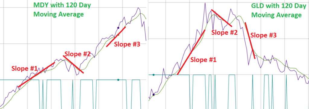
The slope of the moving average is the rate of change of the moving averages over the period of time selected. Our Rotation Advanced Tool allows the user to define the length of the moving average.
This is best represented with a visual chart as the fund with the greater positive slope of the moving average of the price. As you can see below there are. Our tools use a moving average input by the user (ex. 120 days shown below), and at the end of the month determine which has the better (more positive) rate of change – visually the rate of change is the slope of the moving average line.
In the example below the 120 Day Moving average is being compared between MDY and GLD at 3 different points. For Point #1 (Slope #1), visually GLD has the large (steeper) slope, thus the greater rate of change, and is the winner of Point #1. For Point #2 (Slope #2), visually GLD has the less negative (less steep negative) slope, thus the greater rate of change even though both are negative, and is the winner of Point #2. For Point #3 (Slope #3), visually GLD has the negative slope and MDY has a positive slope, thus the greater rate of change is MDY, and is the winner of Point #3.
Frequency of Updates
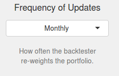
The frequency of updates is simply how often the backtester re-checks the conditions to determine if it should rotate out of a position or change the allocation or check if a security is above or below the moving average. So for a monthly update (as shown above), the backtester will only look re-calculate every 1 month at the end of the month and rotate or adjust allocation.
Top N and Top N Keep K - Rotation Tools Only
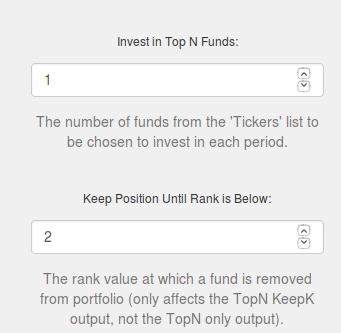
In the Rotation tools (Simple and Advanced), you may select how many funds the rotation tool invests in (top n), and if the rotation tool should hold onto the funds until it drops a certain distance in the rankings (keep k).
Top N: This is how many funds the rotation tool will select from the list each period and invest in.
Keep K: This is how far a fund has to drop in the position score ranking before it will be sold at which point it will be replaced by the fund with the highest ranking.
Cash Filter Calculations
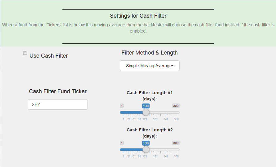
The cash filter may be used on the Rotation and Moving Average Tools as well as the Volatility Target tool. If a fund’s price is below the moving average(s) that fund will be replaced with the Cash Filter Fund Ticker entered on this page. The moving average Filter Method may be selected using different types of moving average calculations. The length may be set to values between 1 and 300, and denotes the number of trading days to do a calculation on.
As an example, if the price of the fund SPY is currently 200, and the value of the 100 day moving average is 201 then at the next period update SPY is below the moving average and therefore instead of investing in SPY the backtester will invest in the cash filter fund selected. Alternatively if the fund SPY is currently 200, and the value of the 100 day moving average is 180 then at the next period update SPY is above the moving average and therefore the cash filter will do nothing thus allowing SPY as a valid option to invest in. If any one of the top funds is below the filter it will invest in the cash filter instead of the selected fund.
The Advanced Rotation Tool allows the user to select 2 different moving average lengths, if a fund is below either moving average then the backtester will invest in the Cash Filter Fund Ticker. Keep in mind the condition for how often to check if a fund is below the moving average (and thus switch it out for the cash filter fund) is only evaluated based on the update frequency described above.
Adaptive Asset Allocation Weighting Calculations
In tools that offer Adaptive Asset Allocation, the algorithm for finding position sizing is: Current Ticker’s Value / Sum of all values
Example of determining weights for a 3 month Sharpe Ratio based Adaptive Asset Allocation:
SPY has a Sharpe ratio of 1.3
MDY has a Sharpe ratio of 1.7
TLT has a Sharpe ratio of 0.3
GLD has a Sharpe ratio of -0.4 [this is rounded to 0 for calculation purposes]
Sum of all Sharpe Values = 1.3 + 1.7 + 0.3 + 0 [rounded to 0 for calculations] = 3.3
Formula: Current Ticker’s Value / Sum of all values
SPY Weight = 1.3 / 3.3 = 39.4%
MDY Weight = 1.7 / 3.3 = 51.5%
TLT Weight = 0.3 / 3.3 = 9.1%
GLD Weight = 0 / 3.3 = 0%
Position Score Calculations [For Rotation Tools]
What our tools do is take the lowest momentum fund in the list, then rank it from 1 to xx for mean reversion. Once it is ranked we then take all the rankings and multiply them by there
Example (60% 3-month Momentum, 40% 10 day Mean Reversion):
Fund A has a 3-month Momentum of 6% and a 10 day Mean Reversion of -3%. Thus Fund A is Rank 1 for Mean Reversion and Rank 2 for Momentum.
Fund B has a 3-month Momentum of 7% and a 10 day Mean Reversion of 0%. Thus Fund B is Rank 2 for Mean Reversion and Rank 1for Momentum.
Score for Fund A = 60% * 1 + 40% * 2 = 1.4
Score for Fund B = 60% * 2+ 40% * 1= 1.6
–> Thus Fund A has the lower score, and is chosen as the winner. This is because 3-month Momentum was selected as being more important (60%) than Mean Reversion (40%).
[In event of a tie, a fund is randomly chosen]
Adjusted Close Prices for Funds (for Dividends and Splits)
Update frequency
Data for most US equities are updated by 5:30pm EST everyday, with our caching updates may come as late as 7:30PM EST. Mutual funds and ETFs are updated by 12AM for the previous day.
Redundancy and Automated Checking
Each feed is made up of at least 3 data sources on average. This means if any one of them goes down, you keep going. Secondly, this let’s us implement error-checking and catch missing data and erroneous data-points.
Adjusted Data
A company may undergo splits and dividends, which means prices may not accurately reflect the real value of a company. Adjusted data takes this into consideration.
Some data adjustments are not available. In those situations, values will be null.
Cash Dividends
If a company’s share price $100/share, and they issue a $1 share/dividend, the share price of a company will fall $1 to reflect this change on the ex-dividend date (they are liquidating the company’s assets for cash to shareholders). The value of the company has not fallen 1% (they just converted equity to cash), but the share price will fall by 1%. Therefore, we need to adjust the Open, High, Low, and Close values by $1.
The formula for this adjustment is:
Adjustment Ratio = (Close Price + Dividend Amount) / (Close Price)
Some data adjustments are not available. In those situations, values will be null.
For ADRs that pay distributions in Non-USD: For US-listed ADRs that pay their dividends in Non-USD (e.g. OSB), we automatically convert the distribution to USD before applying the adjustments. The dividend amount will also be the dividend in USD.
Stock Dividends
Instead of cash, a company may issue dividends in Stock. For example a 1% stock dividend, means a shareholder may receive 1 share for every 100 shares they own.
The formula for this adjustment is:
Adjustment Ratio = (New Float) / (Old Float)
Where float is the number of shares issued by the company.
Splits
When a company splits, or reverse splits, the data is also backward adjusted. For example in a 5:1 split (5 for 1), 1 share becomes 5. In this case the split Factor will be 5. In a reverse split, for example 1:10 (1 for 10), 10 shares become 1 share. In this case, the split Factor will be 0.10.
Therefore, the formula for this adjustment is:
Adjustment Ratio = (To split factor) / (For Split Factor)
a regular 5:1 split reads, 5 shares for 1 share.
Spinoffs
Spinoffs are treated by assuming you sell off the shares of the company that was spun off at the opening price, and use the proceeds to buy back the original stock at the opening price.
The formula for this adjustment is:
Adjustment Ratio = 1 + (Spinoff Open Price * Spinoff Shares) / (Parent Open Price * Parent